Benchmarks

In the same way that using R packages cpp11 or Rcpp allows you to bridge your R code with C++ code that runs faster than R, you can use luajr to bridge your R code with Lua code that runs faster than R.

Often, C/C++ code runs about 5-100 times faster than the equivalent R code. In my experience, luajr code typically presents a similar speedup. The amount of speedup also depends strongly on what you’re doing.

Why use luajr then? Rcpp and cpp11 require a C++ toolchain (e.g.  gcc, clang, etc.) and requires long compilation times, whereas luajr doesn’t. This means that luajr is usable when a C++ compiler isn’t available, or when compilation times are prohibitive or an annoyance.

In this vignette, we show a few example benchmarks to show situations where luajr offers a substantial improvement in code execution speed and when it doesn’t.

Example 1: when to stick with R

Lots of R’s built-in functions are already speedy because they rely on compiled C code. For example, consider the following ways you might sum all the elements of a numeric vector:

library(luajr)

x <- rnorm(1e6)

# Method one: built-in sum
s1 <- sum(x)

# Method two: sum in R
sum_R <- function(x) {
    s <- 0
    for (y in x) {
        s <- s + y
    }
    return (s)
}
s2 <- sum_R(x)

# Method three: sum in Lua
sum_L <- lua_func("function(x)
    local s = 0
    for i = 1, #x do
        s = s + x[i]
    end
    return s
end")
s3 <- sum_L(x)

Each method produces the same answer. Using bench::mark() on a 2025-era MacBook Pro, the execution time for each method is as follows:

Method	Median runtime
sum(x)	664 µs
sum_R(x)	6340 µs
sum_L(x)	546 µs

R’s built-in sum() function calls an internal R function written in C, so it is already relatively fast. The “naïve” sum_R() function, which calculates the sum manually, is around 10x slower. And the Lua version just barely edges out R’s built-in sum() function, but it’s worth noting that Lua arithmetic may not handle NA values correctly for numeric vectors and certainly won’t handle NA values correctly for integers (without explicit handling).

Example 2: logistic map

Consider the following:

logistic_map_R = function(x0, burn, iter, A)
{
    result_x = numeric(length(A) * iter)
    
    j = 1
    for (a in A) {
        x = x0
        for (i in 1:burn) { 
            x = a * x * (1 - x)
        }
        for (i in 1:iter) { 
            result_x[j] = x
            x = a * x * (1 - x)
            j = j + 1
        }
    }
    
    return (list2DF(list(a = rep(A, each = iter), x = result_x)))
}

logistic_map_L = lua_func(
"function(x0, burn, iter, A)
    local dflen = #A * iter
    local aa = luajr.numeric(dflen, 0)
    local xx = luajr.numeric(dflen, 0)
    
    local j = 1
    for k, a in pairs(A) do
        local x = x0
        for i = 1, burn do
            x = a * x * (1 - x)
        end
        for i = 1, iter do
            aa[j] = a
            xx[j] = x
            x = a * x * (1 - x)
            j = j + 1
        end
    end
    
    local result = luajr.dataframe()
    result:set('a', aa)
    result:set('x', xx)
    
    return result
end", "native, native, native, auto")

# To be compiled using Rcpp::cppFunction()
logistic_map_C =
'DataFrame logistic_map(double x0, unsigned int burn, unsigned int iter, NumericVector A)
{
    unsigned int dflen = A.length() * iter;
    NumericVector da(dflen, 0);
    NumericVector dx(dflen, 0);
    
    unsigned int j = 0;
    for (auto a : A)
    {
        double x = x0;
        for (unsigned int i = 0; i < burn; ++i)
            x = a * x * (1 - x);
        for (unsigned int i = 0; i < iter; ++i, ++j)
        {
            dx[j] = x;
            da[j] = a;
            x = a * x * (1 - x);
        }
    }

    return DataFrame::create(Named("a") = da, Named("x") = dx);
}'

Here we are comparing three different versions (R, Lua, C++) of running a parameter sweep of the logistic map, a chaotic dynamical system popularized by Bob May in a 1976 Nature article. The output looks like this:

logistic_map = logistic_map_L(0.5, 100, 100, 200:385/100)
plot(logistic_map$a, logistic_map$x, pch = ".")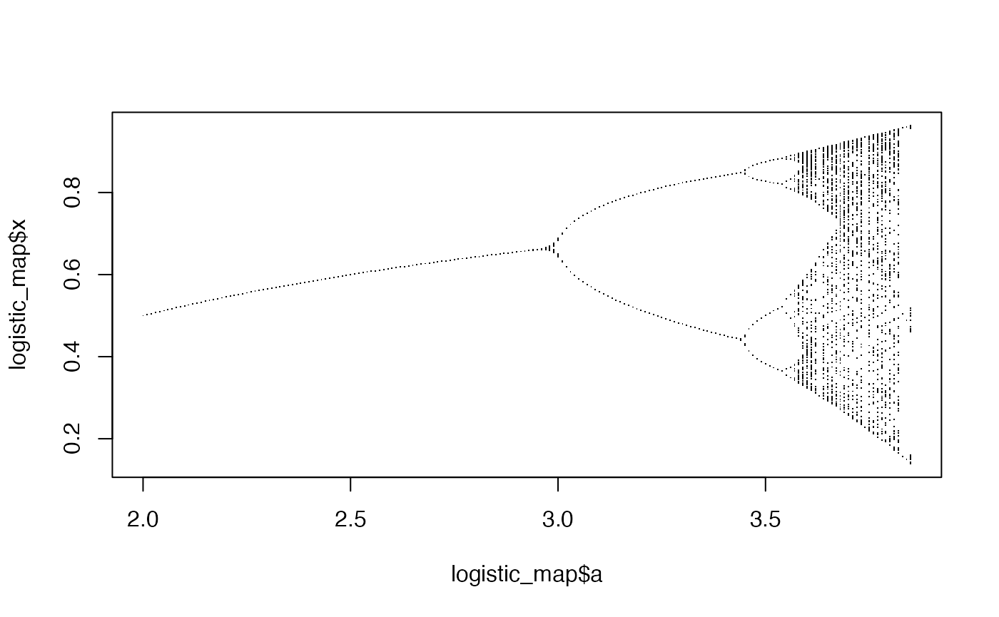

The times taken by each function on a 2025-era MacBook Pro are as follows:

Call	Method	Median runtime
logistic_map_R(0.5, 100, 100, 200:385/100))	R function	850 µs
logistic_map_L(0.5, 100, 100, 200:385/100))	Lua function	80 µs
logistic_map_C(0.5, 100, 100, 200:385/100))	C++ function	100 µs

The version written in Lua is around 10 times faster than the version in R, and even somewhat outperforms Rcpp. Note that the relative speed of Lua versus C++ depends on the number of iterations, and whether you use Rcpp or cpp11, which each seem to have marginal advantages in different cases. Nonetheless, the Lua version seems to execute about as quickly as the C++ version, within plus or minus 20%.

The speedup of the Lua function relative to R was much more notable in an earlier test where the R version first created the data frame and then performed the iteration, i.e. with the line result$x[j] = x instead of result_x[j] = x. The median runtime for that R version was two orders of magnitude slower than the Lua version; the extra overhead associated with data.frame methods was pointed out by Tim Taylor. This goes to show that when aiming for efficient R code, it helps to know a few tricks.

Example 3: Lorenz attractor

Even greater speedups can be seen when conducting more intensive calculations. For example, solving a system of ordinary differential equations (ODEs) is a common scientific task. Normally this is done in R using a general-purpose package such as deSolve. In this benchmark we will instead do simple Euler integration of the famous chaotic Lorenz system.

To calculate this system entirely in R, you might write something like the following:

# Lorenz attractor in R

# Take a single step, size dt, of the Lorenz system
step1 = function(x, rho, sigma, beta, dt)
{
    dx = sigma * (x[2] - x[1])
    dy = x[1] * (rho - x[3]) - x[2]
    dz = x[1] * x[2] - beta * x[3]
    x[1] = x[1] + dx * dt
    x[2] = x[2] + dy * dt
    x[3] = x[3] + dz * dt
    return (x)
}

# Calculate Lorenz system trajectory
lorenz1 = function(n, init, rho, sigma, beta)
{
    x = init
    result = matrix(0, nrow = n, ncol = 3)
    for (i in 1:n) {
        result[i, ] = x
        x = step1(x, rho, sigma, beta, 0.01)
    }
    return (result)
}

# Generate and plot result
result1 = lorenz1(5000, c(1,1,1), 28, 10, 8/3)
plot(result1[,1], result1[,2], type = "l")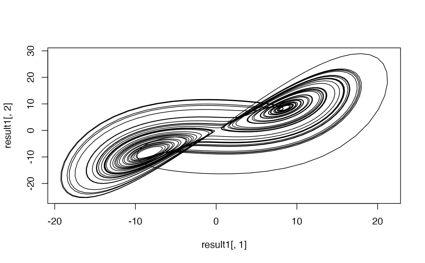

Similar code can be written entirely in Lua using luajr:

# Lorenz attractor in Lua
library(luajr)

lorenz2 = lua_func("
function(n, init, rho, sigma, beta)
    local step2 = function(x, rho, sigma, beta, dt)
        local dx = sigma * (x[2] - x[1])
        local dy = x[1] * (rho - x[3]) - x[2]
        local dz = x[1] * x[2] - beta * x[3]
        x[1] = x[1] + dx * dt
        x[2] = x[2] + dy * dt
        x[3] = x[3] + dz * dt
        return x
    end

    local x = init
    local result = luajr.matrix(n, 3)

    for i = 1,n do
        result[i] = x[1]
        result[i + n] = x[2]
        result[i + 2*n] = x[3]
        x = step2(x, rho, sigma, beta, 0.01)
    end

    return result
end", "native auto native")

result2 = lorenz2(5000, c(1,1,1), 28, 10, 8/3)
plot(result2[,1], result2[,2], type = "l")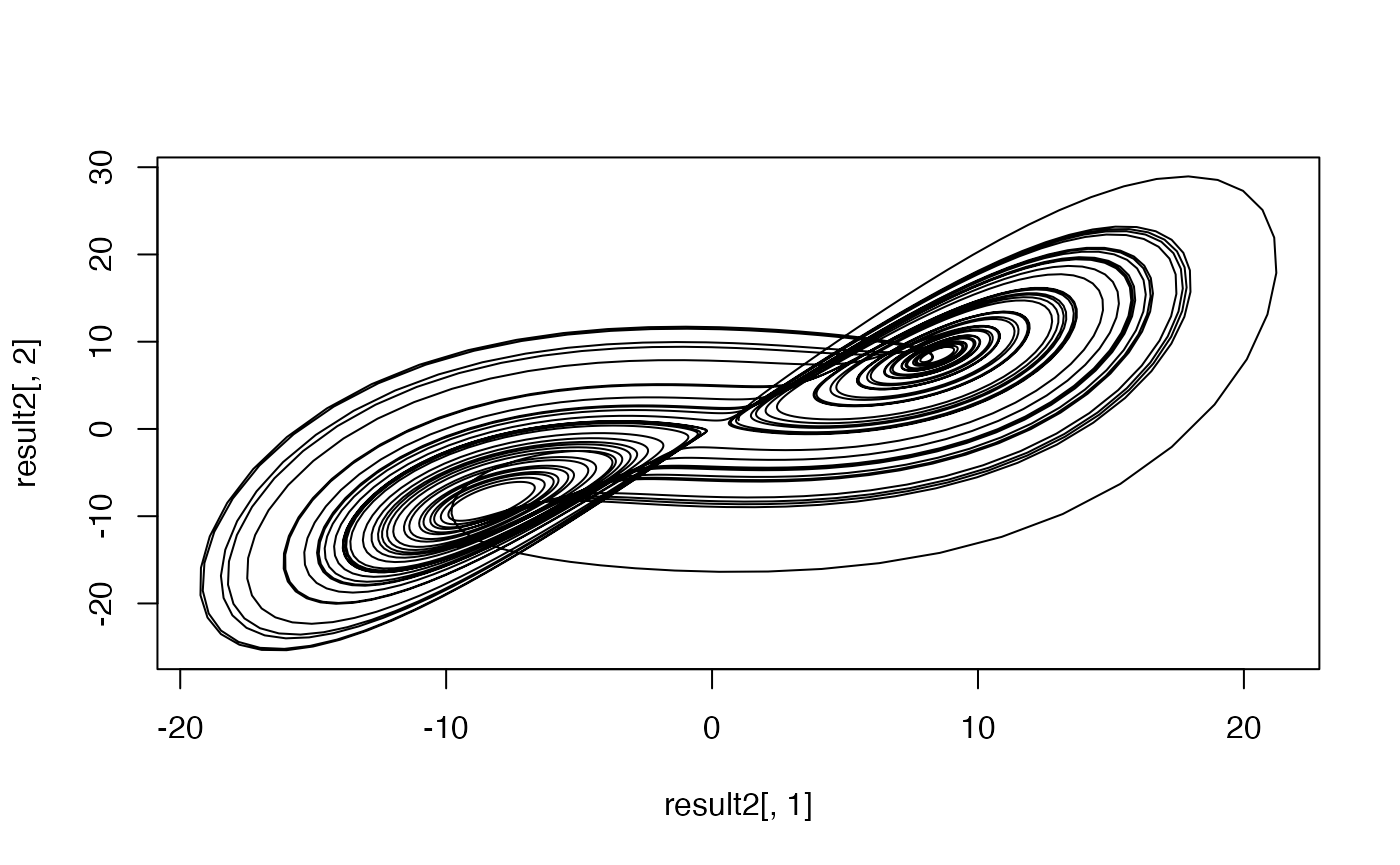

Execution times are as follows:

Call	Method	Median runtime
lorenz1(5000, c(1, 1, 1), 28, 10, 8/3)	R function	3300 µs
lorenz2(5000, c(1, 1, 1), 28, 10, 8/3)	Lua function	38 µs

The Lua code is 85 times faster than the equivalent R code.

As mentioned before, a library such as deSolve is normally used to integrate systems of ODEs and both versions above do execute rather quickly anyway – it may not be worth the trouble here to save 3 milliseconds! But for intensive and complex simulations, it may help to get a substantial speed boost over what base R can do.